Quantum computing works by preparing qubits, applying quantum gates and measuring the resulting state. A useful algorithm arranges those operations so interference changes the probabilities of outcomes that carry an answer.
The processor does not return every possible answer at once. Measurement produces ordinary data, and the program usually needs repeated circuit runs and classical processing to interpret that data.
This guide follows a small circuit from input to output. For the meaning of an individual quantum bit, start with What is a qubit?.
A quantum program starts with a state
A classical program can store bits with values of zero or one. A quantum circuit describes a state using amplitudes associated with possible measurement outcomes. For a single qubit, those outcomes are zero and one when measured in the standard computational basis.
Amplitudes are not simply probabilities. They include phase information, and the probability of an outcome is the squared magnitude of its amplitude. That difference allows quantum operations to change a later measurement in ways a classical random coin cannot reproduce.
You do not need to calculate those amplitudes to read a circuit diagram. Follow the qubit’s starting state, the gates applied to it, and where measurement occurs.
Gates change the state before measurement
A gate is a controlled transformation of the quantum state. In the ideal circuit model, gates are reversible and preserve the total probability of the possible outcomes.
IBM’s quantum mechanics lesson uses the Hadamard gate, labelled H, as an example. Applied to a qubit starting in state zero, it produces an equal superposition of zero and one.
If you immediately measure that qubit in the computational basis, the ideal probabilities are 50% for zero and 50% for one. One run gives one outcome, not both values.
But measurement is not the only next step. You can apply another gate while the quantum state remains available for coherent processing. That is where the circuit begins to behave differently from a sequence of ordinary random choices.
Why two H gates return zero
Consider two circuits starting with a qubit in state zero.
| Ideal circuit | Measurement probabilities |
|---|---|
| Start at zero → H → measure | Zero: 50%; one: 50% |
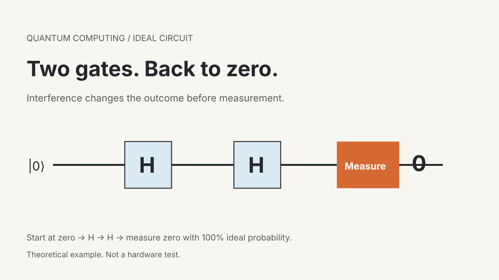
| Start at zero → H → H → measure | Zero: 100%; one: 0% |
These are theoretical results for ideal gates, not results from a hardware test.
The second H gate reverses the first. More precisely, the transformation makes the contributions to the final zero amplitude add together and the contributions to the one amplitude cancel.
This is interference. Quantum algorithms use the structure of gates and phase relationships to favour useful outcomes and suppress others. Describing a quantum computer as “trying every answer simultaneously” leaves out the problem of arranging that interference and extracting useful information.
A second coin toss would not undo the randomness of a first coin toss. The first H gate has not already performed a measurement or selected a classical random bit. Treating those two operations as equivalent misses the part that matters.
Entanglement connects multiple qubits
With more qubits, some states cannot be described as independent states for each qubit. Such states are entangled.
IBM’s lesson constructs a Bell state by applying H to one qubit and then a controlled-X gate between two qubits. In that ideal example, measuring the pair in the computational basis produces either 00 or 11, with equal probability.
The individual results are correlated: a zero on one accompanies a zero on the other. The joint state describes the pair.
That does not mean every quantum circuit must look like this example. It also does not provide a way to send a chosen message instantaneously. The Bell circuit is a small illustration of the joint-state relationships that quantum operations can create.
For a larger circuit, the algorithm must control those relationships alongside interference and the measurement strategy. Counting qubits alone does not describe what the program can accomplish.
Measurement returns classical information
Measurement converts the relevant quantum information into a recorded outcome. In the simple single-qubit example, that is a zero or a one. It does not expose a list of all the amplitudes in one run.
Programs often repeat a circuit many times. Each run is commonly called a shot. The collected outcomes provide information about the circuit’s measurement distribution, which classical software can analyse.
For example, an ideal equal-superposition circuit predicts a 50/50 distribution. A finite collection of shots need not contain exactly half zeros and half ones. Random sampling alone can produce variation; on hardware, implementation errors can also affect the distribution.
Distinguish three things in any reported result: the ideal mathematical prediction, a simulation, and execution on a physical device. They answer different questions. Neither a circuit drawing nor an ideal simulator output establishes a device’s performance.
Why an algorithm is more than a circuit demo
An H gate example demonstrates a mechanism. It does not show that a quantum computer can solve an arbitrary business problem faster than a classical computer.
A useful computation needs a way to encode the problem, choose transformations, measure relevant quantities and interpret the output. Its practical cost also includes repeated execution and the classical work surrounding the circuit.
The particular problem matters. A speed claim needs to identify the task, the comparison method, the resources used and the conditions of the experiment. “Quantum” by itself is not evidence of an advantage.
When reading a launch announcement, separate the number of physical qubits from the circuit that ran and the task it performed. A demonstration of a state or a gate is not automatically a demonstration of a useful end-to-end calculation.
The classical computer remains part of the process
Classical software defines circuits, manages inputs and processes measured outcomes. A quantum processor is one component of the computing workflow, not a replacement for every part of an ordinary computer.
This also explains why quantum computation and quantum-safe encryption are separate subjects. One concerns processing information with quantum systems; the other concerns cryptographic protections designed for threats that include sufficiently capable quantum computers. Read post-quantum cryptography explained for that distinction.
A clear account of quantum computing should make the route to the answer visible: preparation, gates, interference, measurement and interpretation. If a claim stops at “many possibilities,” ask how the program obtains the useful output.
Sources
IBM Quantum Learning, Quantum mechanics basics, consulted October 7, 2026. The single-qubit probabilities are ideal theoretical examples derived from the documented Hadamard transformation, not hardware measurements.